Introduction:
Survival Analysis is a statistical approach that enables the examination of event occurrence rates over time without assuming these rates remain constant. Principally, it facilitates modeling the duration until an event’s occurrence, comparison of such durations across diverse groups, or the investigation of the relationship between time-to-event and quantitative variables. This method is particularly adept at handling censored data, a scenario where the event of interest (such as death, failure, or recovery) hasn’t occurred for some subjects during the study period.
Hazard Function represents the instant rate of event occurrence at a given time point, t. Unlike the assumption of constant hazard rates in some analyses, survival analysis recognizes the variability of these rates over time. The cumulative hazard then aggregates the hazard experienced until time t.
Survival Function is defined as the likelihood of an individual’s survival—or alternatively, the non-occurrence of the event of interest—up to a certain point in time, t. Mathematically, it’s depicted as , with representing a probability value between 0 and 1, given that survival times are non-negative ().
Kaplan-Meier Curve visualizes the survival function as a step function, marking the cumulative probability of survival over time. It remains horizontal during intervals without events, dropping at points where events occur, reflecting changes in the survival function.
Censoring in Survival Analysis is a unique aspect concerning missing data wherein the event of interest is not observed for certain subjects by the study’s end, either due to their withdrawal or other non-event-related reasons. The predominant form encountered is right censoring, with left censoring occurring when the start time is unknown.
hazard ratio (HR) is the key metric derived from a Cox regression analysis. This ratio quantifies the comparative hazards between two distinct groups at any given moment. It reflects the instant rate at which the event of interest occurs among those still susceptible to it. Importantly, it should not be construed as a measure of risk, although it is frequently misunderstood in this way. For a regression coefficient , the hazard ratio is computed as HR = .
An HR less than 1 suggests a lower hazard of the event under study, typically death, for the group in question compared to the reference group. Conversely, an HR greater than 1 indicates a higher hazard of the event for the group in question. Thus, an HR of 0.59 would mean that the hazard for females is 0.59 times that for males at any specific time point, signifying that females have a markedly lower hazard of death compared to males according to the dataset.
Proportional Hazards Assumption is fundamental to comparing survival functions across groups, such as different patient cohorts, this assumption does not necessitate constant hazards but maintains a constant hazard ratio over time, enabling comparisons of hazard rates across different observation periods.
Survival objects:
IPD_data <- NeuroblastomaPSM::IPD_data
# Split IPD by curves and treatments:
IPD_curves_trts <- split(
  x = IPD_data,
  f = interaction(IPD_data$trt, IPD_data$curve)
)

lapply(
  X = names(IPD_curves_trts) |>
    `names<-`(names(IPD_curves_trts)),
  FUN = function(surv_data_nm) {
    print(gsub("\\.", " ", surv_data_nm))

    surv_data <- IPD_curves_trts[[surv_data_nm]]
    print(rbind(head(surv_data, n = 5), tail(surv_data, n = 5)))
  }
) |>
  invisible()
#> [1] "Dinutuximab β EFS"
#>               trt trt_cd curve eventtime event
#> 425 Dinutuximab β    GD2   EFS     0.013     1
#> 426 Dinutuximab β    GD2   EFS     0.013     1
#> 427 Dinutuximab β    GD2   EFS     0.013     1
#> 428 Dinutuximab β    GD2   EFS     0.013     1
#> 429 Dinutuximab β    GD2   EFS     0.046     1
#> 620 Dinutuximab β    GD2   EFS     7.000     0
#> 621 Dinutuximab β    GD2   EFS     7.000     0
#> 622 Dinutuximab β    GD2   EFS     7.000     0
#> 623 Dinutuximab β    GD2   EFS     7.000     0
#> 624 Dinutuximab β    GD2   EFS     7.000     0
#> [1] "Isotretinoin EFS"
#>              trt trt_cd curve   eventtime event
#> 113 Isotretinoin     TT   EFS  0.03278242     1
#> 114 Isotretinoin     TT   EFS  0.03278242     1
#> 115 Isotretinoin     TT   EFS  0.04538207     1
#> 116 Isotretinoin     TT   EFS  0.07793117     1
#> 117 Isotretinoin     TT   EFS  0.12202994     1
#> 220 Isotretinoin     TT   EFS 14.70647482     0
#> 221 Isotretinoin     TT   EFS 14.70647482     0
#> 222 Isotretinoin     TT   EFS 14.70647482     0
#> 223 Isotretinoin     TT   EFS 14.70647482     0
#> 224 Isotretinoin     TT   EFS 14.70647482     0
#> [1] "Dinutuximab β OS"
#>               trt trt_cd curve eventtime event
#> 225 Dinutuximab β    GD2    OS 0.1504637     1
#> 226 Dinutuximab β    GD2    OS 0.1985816     1
#> 227 Dinutuximab β    GD2    OS 0.2908074     1
#> 228 Dinutuximab β    GD2    OS 0.2908074     1
#> 229 Dinutuximab β    GD2    OS 0.3212821     1
#> 420 Dinutuximab β    GD2    OS 6.9671577     0
#> 421 Dinutuximab β    GD2    OS 6.9671577     0
#> 422 Dinutuximab β    GD2    OS 6.9671577     0
#> 423 Dinutuximab β    GD2    OS 6.9671577     0
#> 424 Dinutuximab β    GD2    OS 6.9671577     0
#> [1] "Isotretinoin OS"
#>              trt trt_cd curve   eventtime event
#> 1   Isotretinoin     TT    OS  0.09677419     1
#> 2   Isotretinoin     TT    OS  0.30162856     1
#> 3   Isotretinoin     TT    OS  0.38686900     1
#> 4   Isotretinoin     TT    OS  0.38686900     1
#> 5   Isotretinoin     TT    OS  0.44697776     1
#> 108 Isotretinoin     TT    OS 14.72539931     0
#> 109 Isotretinoin     TT    OS 14.72539931     0
#> 110 Isotretinoin     TT    OS 14.72539931     0
#> 111 Isotretinoin     TT    OS 14.72539931     0
#> 112 Isotretinoin     TT    OS 14.72539931     0

# Split IPD by curves:
IPD_curves <- split(
  x = IPD_data,
  f = IPD_data$curve
)
Utilizing the {survival} package, the Surv() function
generates a survival object suitable for being the response in a model’s
formula. Each subject is represented by their survival time in this
object, with censored subjects marked by a +. Here’s a
glimpse at the reconstructed individual patient data (IPD):
lapply(
  X = names(IPD_curves_trts) |>
    `names<-`(names(IPD_curves_trts)),
  FUN = function(trt_curve_nm) {
    surv_data <- IPD_curves_trts[[trt_curve_nm]]
    surv_obj <- survival::Surv(
      time = surv_data$eventtime,
      event = surv_data$event
    )

    print(gsub("\\.", " ", trt_curve_nm))

    print(
      c(head(surv_obj, n = 5), tail(surv_obj, n = 5))
    )
  }
) |>
  invisible()
#> [1] "Dinutuximab β EFS"
#>  [1] 0.013  0.013  0.013  0.013  0.046  7.000+ 7.000+ 7.000+ 7.000+ 7.000+
#> [1] "Isotretinoin EFS"
#>  [1]  0.03278242   0.03278242   0.04538207   0.07793117   0.12202994
#>  [6] 14.70647482+ 14.70647482+ 14.70647482+ 14.70647482+ 14.70647482+
#> [1] "Dinutuximab β OS"
#>  [1] 0.1504637  0.1985816  0.2908074  0.2908074  0.3212821  6.9671577+
#>  [7] 6.9671577+ 6.9671577+ 6.9671577+ 6.9671577+
#> [1] "Isotretinoin OS"
#>  [1]  0.09677419   0.30162856   0.38686900   0.38686900   0.44697776
#>  [6] 14.72539931+ 14.72539931+ 14.72539931+ 14.72539931+ 14.72539931+
Non-Parametric Methods: Kaplan-Meier Curves
The Kaplan-Meier method is a cornerstone of survival analysis, offering a straightforward way to estimate survival probabilities without assuming a specific statistical distribution for the event times. This method employs a non-parametric technique to produce a step function that decreases each time an event is observed.
To construct survival curves employing the Kaplan-Meier method, one
can use the survfit() function. By applying this function,
a survival curve for each treatment is created.
Kaplan-Meier estimeates:
# KM curves:
survival_curves_estimates <- lapply(
  X = names(IPD_curves_trts) |>
    `names<-`(names(IPD_curves_trts)),
  FUN = function(trt_curve_nm) {
    surv_data <- IPD_curves_trts[[trt_curve_nm]]
    surv_obj <- survival::survfit(
      formula = survival::Surv(time = eventtime, event = event) ~ 1,
      data = IPD_curves_trts[[trt_curve_nm]],
      type = "kaplan-meier",
      conf.type = "log-log"
    )
    cat("\n")
    print(trt_curve_nm)
    print(
      x = surv_obj,
      print.rmean = TRUE
    )
  }
)
#>
#> [1] "Dinutuximab β.EFS"
#> Call: survfit(formula = survival::Surv(time = eventtime, event = event) ~
#>     1, data = IPD_curves_trts[[trt_curve_nm]], type = "kaplan-meier",
#>     conf.type = "log-log")
#>
#>        n events rmean* se(rmean) median 0.95LCL 0.95UCL
#> [1,] 200     92   4.21     0.217     NA    2.64      NA
#>     * restricted mean with upper limit =  7
#>
#> [1] "Isotretinoin.EFS"
#> Call: survfit(formula = survival::Surv(time = eventtime, event = event) ~
#>     1, data = IPD_curves_trts[[trt_curve_nm]], type = "kaplan-meier",
#>     conf.type = "log-log")
#>
#>        n events rmean* se(rmean) median 0.95LCL 0.95UCL
#> [1,] 112     62   7.22     0.645   1.97    1.34      NA
#>     * restricted mean with upper limit =  14.7
#>
#> [1] "Dinutuximab β.OS"
#> Call: survfit(formula = survival::Surv(time = eventtime, event = event) ~
#>     1, data = IPD_curves_trts[[trt_curve_nm]], type = "kaplan-meier",
#>     conf.type = "log-log")
#>
#>        n events rmean* se(rmean) median 0.95LCL 0.95UCL
#> [1,] 200     71   5.02      0.19     NA      NA      NA
#>     * restricted mean with upper limit =  6.97
#>
#> [1] "Isotretinoin.OS"
#> Call: survfit(formula = survival::Surv(time = eventtime, event = event) ~
#>     1, data = IPD_curves_trts[[trt_curve_nm]], type = "kaplan-meier",
#>     conf.type = "log-log")
#>
#>        n events rmean* se(rmean) median 0.95LCL 0.95UCL
#> [1,] 112     53   8.93     0.588     NA    4.41      NA
#>     * restricted mean with upper limit =  14.7
Kaplan-Meier plots:
# KM curves:
survival_curves_km <- lapply(
  X = names(IPD_curves_trts) |>
    `names<-`(names(IPD_curves_trts)),
  FUN = function(trt_curve_nm) {
    surv_data <- IPD_curves_trts[[trt_curve_nm]]
    surv_obj <- survival::survfit(
      formula = survival::Surv(time = eventtime, event = event) ~ 1,
      data = IPD_curves_trts[[trt_curve_nm]]
    )
    plot(
      surv_obj,
      main = paste0(
        "Kaplan-Meier Curve for ",
        gsub(
          pattern = "\\.",
          replacement = " ",
          x = trt_curve_nm
        )
      ),
      xlab = "Time (years)",
      ylab = "Survival probability"
    )
  }
)


# KM curves, by treatment:
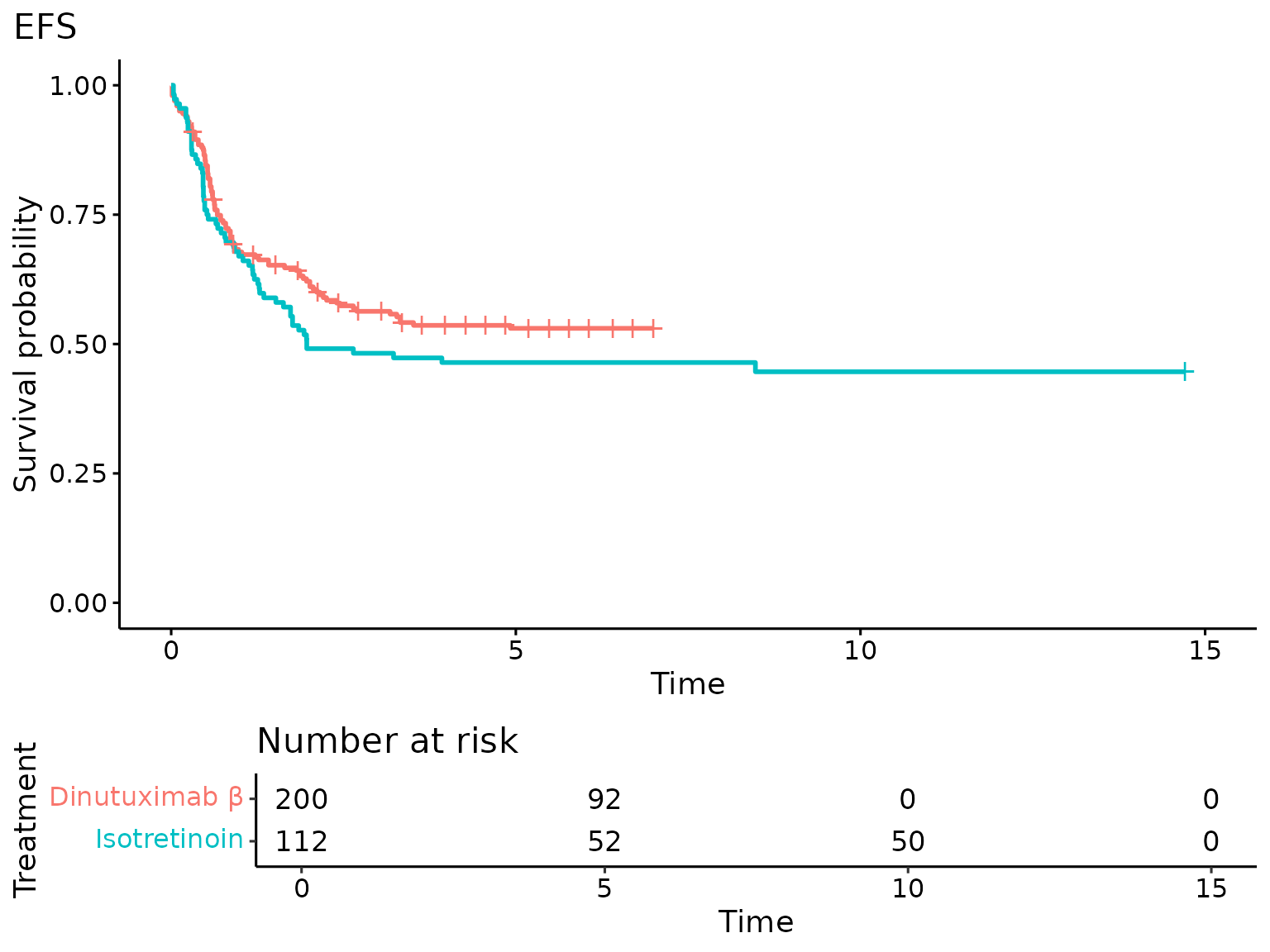
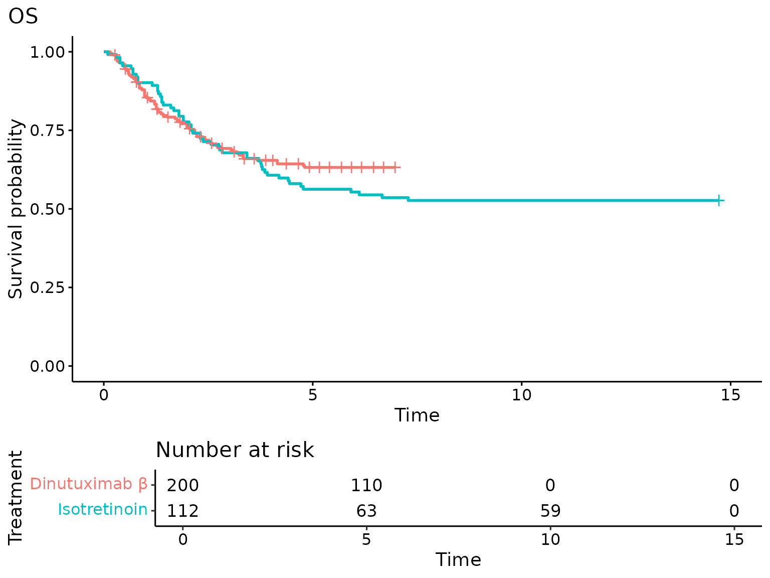
survival_curves_trt_km <- lapply(
X = names(IPD_curves) |>
`names<-`(names(IPD_curves)),
FUN = function(curve_nm) {
surv_obj <- survival::survfit(
formula = survival::Surv(time = eventtime, event = event) ~ trt,
data = IPD_curves[[curve_nm]]
)
surv_plot <- survminer::ggsurvplot(
fit = surv_obj,
data = IPD_curves[[curve_nm]],
risk.table = TRUE,
title = curve_nm,
legend = "none",
legend.title = "Treatment",
legend.labs = unique(IPD_curves[[curve_nm]][["trt"]]) |>
sort()
)
surv_plot$plot <- surv_plot$plot +
ggplot2::theme(plot.title.position = "plot")
print(surv_plot)
surv_obj
}
)
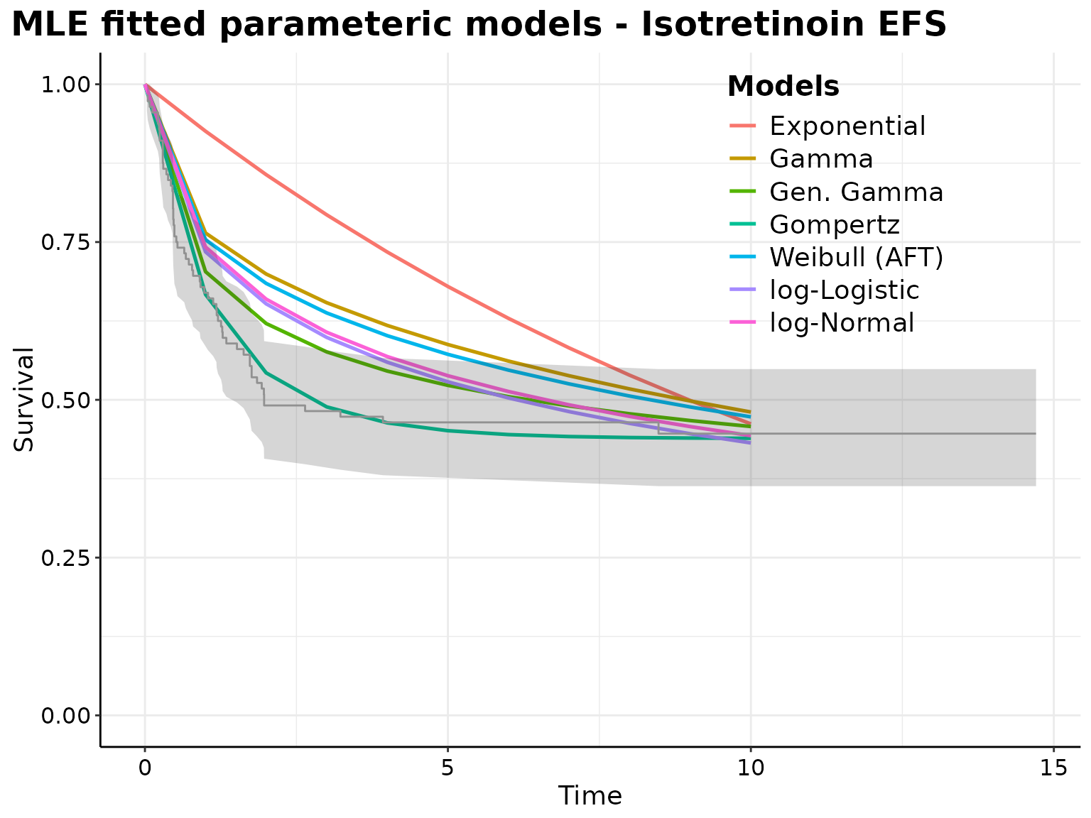
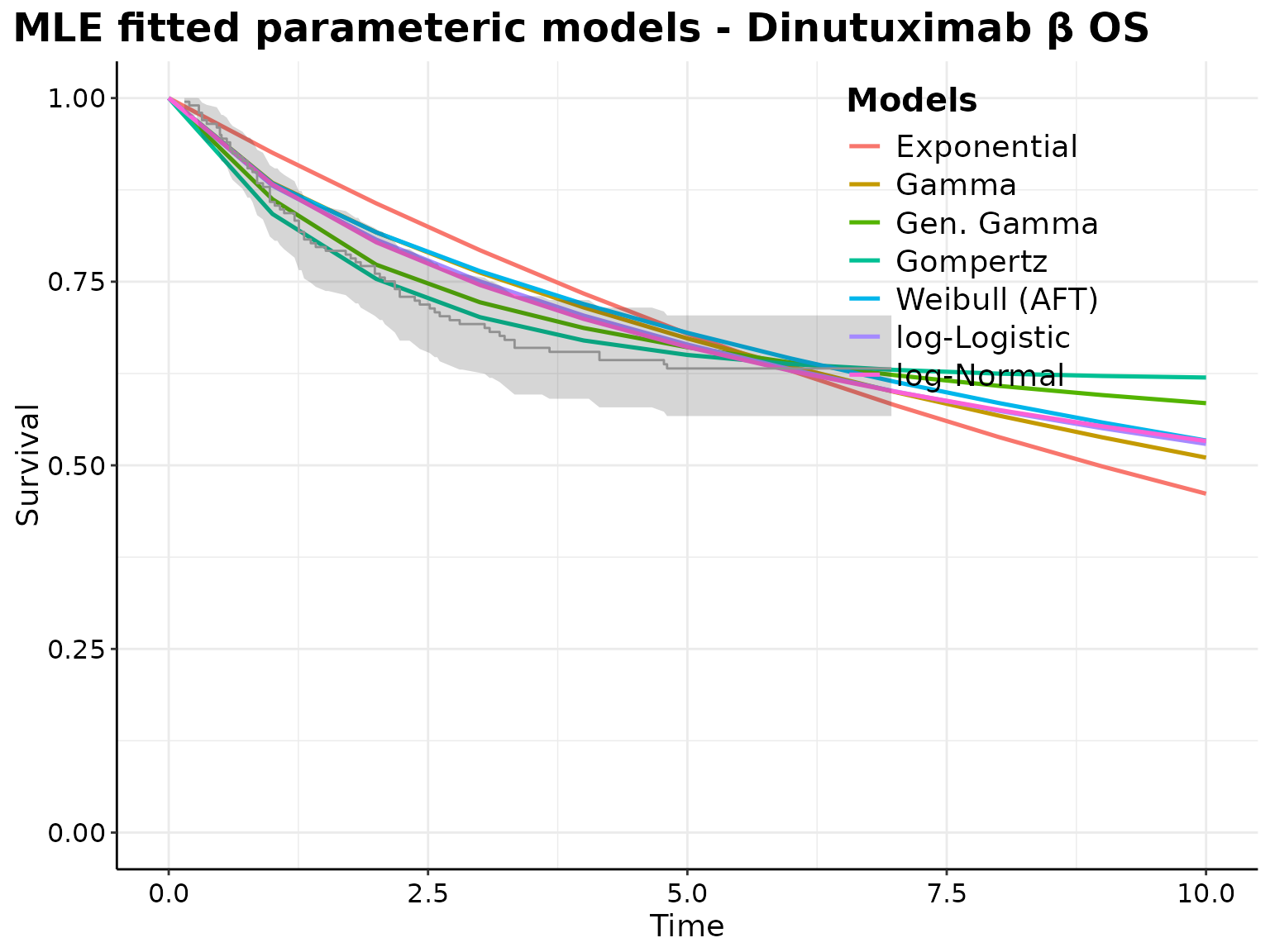
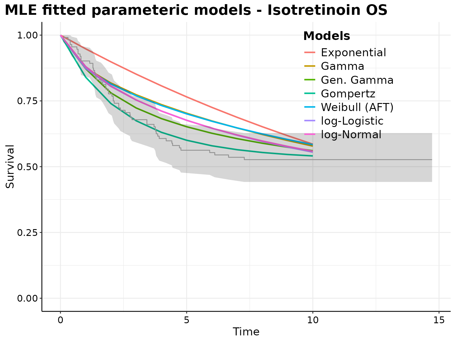
Fitting parametric models:
Parametric models assume a specific statistical distribution for the time-to-event data. This assumption allows for the extrapolation of survival estimates beyond the range of observed data, which is particularly useful in long-term survival predictions where follow-up may not be sufficiently long.
Parametric models using maximum likelihood estimates (MLEs):
Fitting independent survival cuves:
set.seed(1)
# Define models to be used
models <- c("exponential", "gamma", "gengamma", "gompertz", "weibull", "loglogistic", "lognormal")
# Write formula specifying the predictor
formula <- survival::Surv(time = eventtime, event = event) ~ 1
# Fit parametric models:
parametric_models <- lapply(
X = names(IPD_curves_trts) |>
`names<-`(names(IPD_curves_trts)),
FUN = function(curves_trts_nm) {
surv_data <- IPD_curves_trts[[curves_trts_nm]]
surv_parametric_models <- survHE::fit.models(
formula = formula,
data = surv_data,
distr = models,
method = "mle"
)
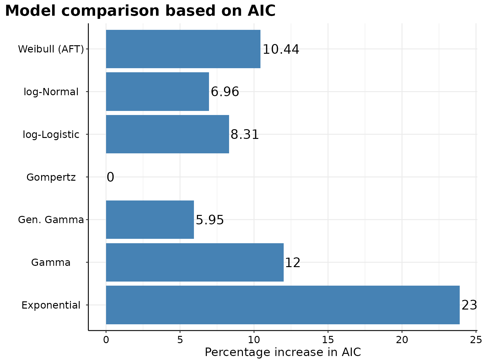
p <- survHE::model.fit.plot(
surv_parametric_models,
scale = "relative"
)
print(
p +
ggplot2::theme(
plot.title.position = "plot",
text = ggplot2::element_text(size = 10),
)
)
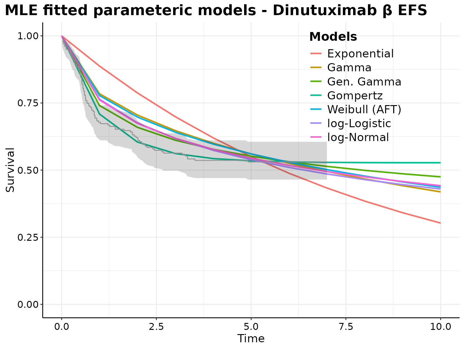
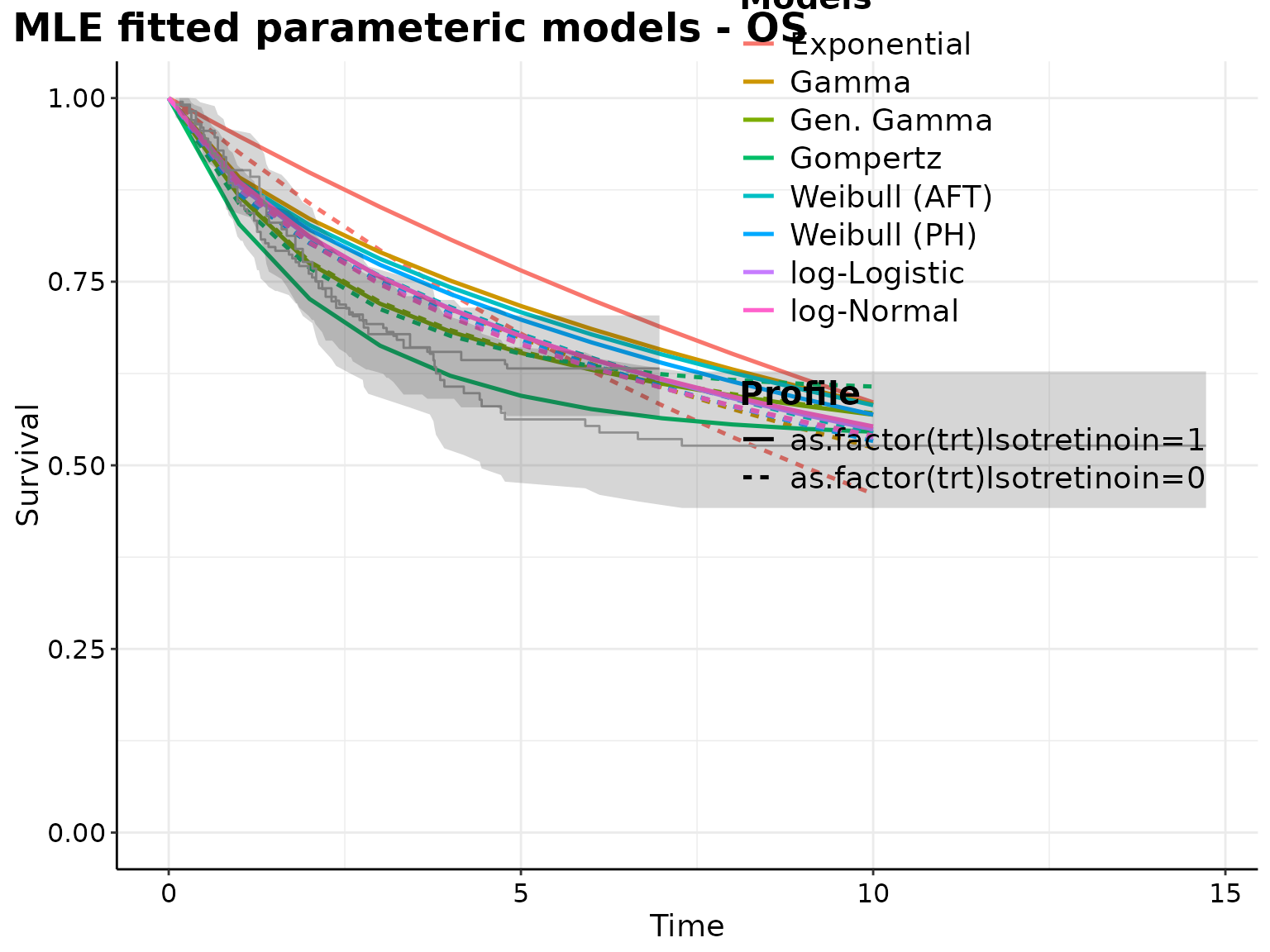
p <- plot(surv_parametric_models, add.km = TRUE, t = seq(0, 10))
print(
p +
ggplot2::labs(
title = paste0(
"MLE fitted parameteric models - ",
gsub(
pattern = "\\.",
replacement = " ",
curves_trts_nm)
)
) +
ggplot2::theme(plot.title.position = "plot")
)
lapply(
X = seq_along(models),
FUN = function(param_model) {
print(surv_parametric_models, mod = param_model)
}
)
surv_parametric_models
}
)
#>
#> Model fit for the Exponential model, obtained using Flexsurvreg
#> (Maximum Likelihood Estimate). Running time: 0.017 seconds
#>
#>          mean        se      L95%    U95%
#> rate 0.118862 0.0123922 0.0968946 0.14581
#>
#> Model fitting summaries
#> Akaike Information Criterion (AIC)....: 577.882
#> Bayesian Information Criterion (BIC)..: 581.180
#>
#>
#> Model fit for the Gamma model, obtained using Flexsurvreg
#> (Maximum Likelihood Estimate). Running time: 0.022 seconds
#>
#>            mean        se      L95%     U95%
#> shape 0.4616622 0.0519674 0.3702611 0.575626
#> rate  0.0275372 0.0086535 0.0148742 0.050981
#>
#> Model fitting summaries
#> Akaike Information Criterion (AIC)....: 522.387
#> Bayesian Information Criterion (BIC)..: 528.984
#>
#>
#> Model fit for the Generalised Gamma model, obtained using Flexsurvreg
#> (Maximum Likelihood Estimate). Running time: 0.031 seconds
#>
#>            mean       se      L95%      U95%
#> mu     0.775818 0.508490 -0.220805  1.772440
#> sigma  3.024955 0.237000  2.594351  3.527030
#> Q     -1.137416 0.410403 -1.941791 -0.333042
#>
#> Model fitting summaries
#> Akaike Information Criterion (AIC)....: 494.155
#> Bayesian Information Criterion (BIC)..: 504.050
#>
#>
#> Model fit for the Gompertz model, obtained using Flexsurvreg
#> (Maximum Likelihood Estimate). Running time: 0.011 seconds
#>
#>            mean        se      L95%      U95%
#> shape -0.771794 0.0969359 -0.961785 -0.581803
#> rate   0.488828 0.0706664  0.368217  0.648946
#>
#> Model fitting summaries
#> Akaike Information Criterion (AIC)....: 466.408
#> Bayesian Information Criterion (BIC)..: 473.004
#>
#>
#> Model fit for the Weibull AF model, obtained using Flexsurvreg
#> (Maximum Likelihood Estimate). Running time: 0.007 seconds
#>
#>            mean        se     L95%      U95%
#> shape  0.515831 0.0486057 0.428845  0.620461
#> scale 13.958535 3.2335174 8.864569 21.979716
#>
#> Model fitting summaries
#> Akaike Information Criterion (AIC)....: 515.124
#> Bayesian Information Criterion (BIC)..: 521.720
#>
#>
#> Model fit for the log-Logistic model, obtained using Flexsurvreg
#> (Maximum Likelihood Estimate). Running time: 0.007 seconds
#>
#>           mean        se     L95%     U95%
#> shape 0.631024 0.0570624 0.528535 0.753388
#> scale 6.222788 1.4408348 3.952723 9.796561
#>
#> Model fitting summaries
#> Akaike Information Criterion (AIC)....: 505.164
#> Bayesian Information Criterion (BIC)..: 511.761
#>
#>
#> Model fit for the log-Normal model, obtained using Flexsurvreg
#> (Maximum Likelihood Estimate). Running time: 0.007 seconds
#>
#>            mean       se    L95%    U95%
#> meanlog 1.90977 0.244549 1.43047 2.38908
#> sdlog   2.68246 0.224748 2.27623 3.16119
#>
#> Model fitting summaries
#> Akaike Information Criterion (AIC)....: 498.888
#> Bayesian Information Criterion (BIC)..: 505.485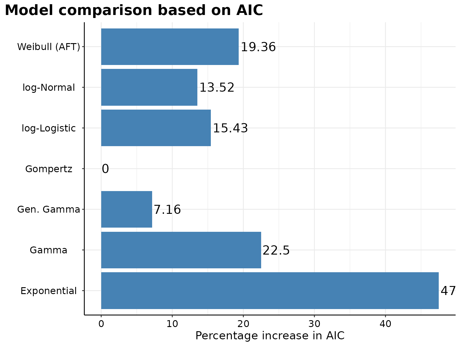
#>
#> Model fit for the Exponential model, obtained using Flexsurvreg
#> (Maximum Likelihood Estimate). Running time: 0.006 seconds
#>
#>           mean         se      L95%     U95%
#> rate 0.0766774 0.00973803 0.0597812 0.098349
#>
#> Model fitting summaries
#> Akaike Information Criterion (AIC)....: 444.450
#> Bayesian Information Criterion (BIC)..: 447.169
#>
#>
#> Model fit for the Gamma model, obtained using Flexsurvreg
#> (Maximum Likelihood Estimate). Running time: 0.018 seconds
#>
#>            mean         se       L95%      U95%
#> shape 0.3522684 0.04824272 0.26934117 0.4607281
#> rate  0.0114968 0.00475699 0.00510951 0.0258687
#>
#> Model fitting summaries
#> Akaike Information Criterion (AIC)....: 369.127
#> Bayesian Information Criterion (BIC)..: 374.564
#>
#>
#> Model fit for the Generalised Gamma model, obtained using Flexsurvreg
#> (Maximum Likelihood Estimate). Running time: 0.025 seconds
#>
#>            mean       se     L95%      U95%
#> mu    -0.431465 0.443078 -1.29988  0.436951
#> sigma  2.367955 0.266802  1.89875  2.953111
#> Q     -2.138324 0.440109 -3.00092 -1.275727
#>
#> Model fitting summaries
#> Akaike Information Criterion (AIC)....: 322.903
#> Bayesian Information Criterion (BIC)..: 331.058
#>
#>
#> Model fit for the Gompertz model, obtained using Flexsurvreg
#> (Maximum Likelihood Estimate). Running time: 0.010 seconds
#>
#>            mean        se      L95%      U95%
#> shape -0.676088 0.0959712 -0.864188 -0.487988
#> rate   0.549287 0.0935185  0.393440  0.766867
#>
#> Model fitting summaries
#> Akaike Information Criterion (AIC)....: 301.333
#> Bayesian Information Criterion (BIC)..: 306.770
#>
#>
#> Model fit for the Weibull AF model, obtained using Flexsurvreg
#> (Maximum Likelihood Estimate). Running time: 0.005 seconds
#>
#>            mean        se      L95%      U95%
#> shape  0.420334 0.0470044  0.337604  0.523337
#> scale 18.841571 6.0402440 10.051673 35.317984
#>
#> Model fitting summaries
#> Akaike Information Criterion (AIC)....: 359.662
#> Bayesian Information Criterion (BIC)..: 365.099
#>
#>
#> Model fit for the log-Logistic model, obtained using Flexsurvreg
#> (Maximum Likelihood Estimate). Running time: 0.008 seconds
#>
#>          mean        se     L95%      U95%
#> shape 0.55806 0.0599002 0.452185  0.688725
#> scale 5.81790 1.8848386 3.083193 10.978223
#>
#> Model fitting summaries
#> Akaike Information Criterion (AIC)....: 347.842
#> Bayesian Information Criterion (BIC)..: 353.279
#>
#>
#> Model fit for the log-Normal model, obtained using Flexsurvreg
#> (Maximum Likelihood Estimate). Running time: 0.006 seconds
#>
#>            mean       se    L95%    U95%
#> meanlog 1.88720 0.317390 1.26512 2.50927
#> sdlog   2.88844 0.293455 2.36692 3.52486
#>
#> Model fitting summaries
#> Akaike Information Criterion (AIC)....: 342.065
#> Bayesian Information Criterion (BIC)..: 347.502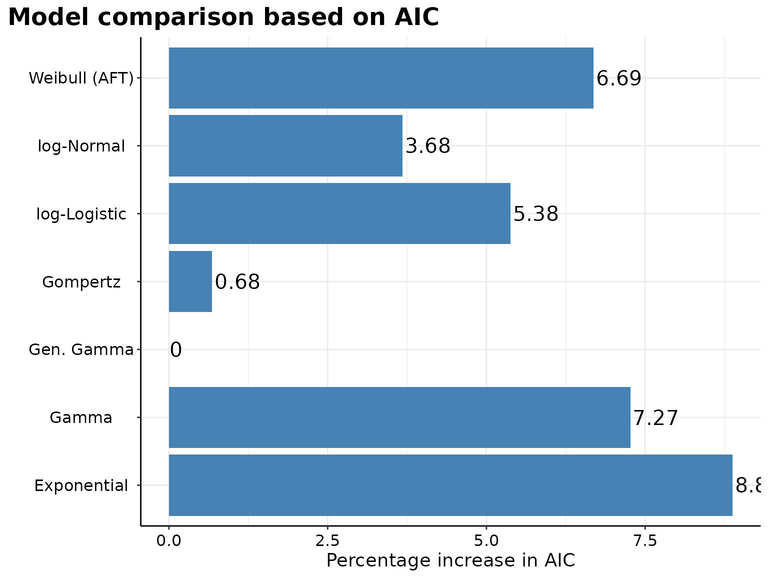
#>
#> Model fit for the Exponential model, obtained using Flexsurvreg
#> (Maximum Likelihood Estimate). Running time: 0.005 seconds
#>
#>           mean         se      L95%      U95%
#> rate 0.0767895 0.00911324 0.0608531 0.0968994
#>
#> Model fitting summaries
#> Akaike Information Criterion (AIC)....: 508.470
#> Bayesian Information Criterion (BIC)..: 511.768
#>
#>
#> Model fit for the Gamma model, obtained using Flexsurvreg
#> (Maximum Likelihood Estimate). Running time: 0.014 seconds
#>
#>            mean        se      L95%      U95%
#> shape 0.6791529 0.0890740 0.5252047 0.8782265
#> rate  0.0358905 0.0116217 0.0190262 0.0677029
#>
#> Model fitting summaries
#> Akaike Information Criterion (AIC)....: 500.959
#> Bayesian Information Criterion (BIC)..: 507.556
#>
#>
#> Model fit for the Generalised Gamma model, obtained using Flexsurvreg
#> (Maximum Likelihood Estimate). Running time: 0.031 seconds
#>
#>            mean       se      L95%     U95%
#> mu     0.420406 0.384705 -0.333602  1.17441
#> sigma  1.958011 0.232639  1.551246  2.47144
#> Q     -2.835463 0.629894 -4.070032 -1.60089
#>
#> Model fitting summaries
#> Akaike Information Criterion (AIC)....: 467.018
#> Bayesian Information Criterion (BIC)..: 476.913
#>
#>
#> Model fit for the Gompertz model, obtained using Flexsurvreg
#> (Maximum Likelihood Estimate). Running time: 0.010 seconds
#>
#>            mean        se      L95%      U95%
#> shape -0.437065 0.0785317 -0.590984 -0.283146
#> rate   0.208811 0.0365708  0.148141  0.294328
#>
#> Model fitting summaries
#> Akaike Information Criterion (AIC)....: 470.201
#> Bayesian Information Criterion (BIC)..: 476.797
#>
#>
#> Model fit for the Weibull AF model, obtained using Flexsurvreg
#> (Maximum Likelihood Estimate). Running time: 0.005 seconds
#>
#>            mean        se     L95%     U95%
#> shape  0.700754 0.0764506  0.56585  0.86782
#> scale 18.891490 4.1623803 12.26649 29.09459
#>
#> Model fitting summaries
#> Akaike Information Criterion (AIC)....: 498.258
#> Bayesian Information Criterion (BIC)..: 504.855
#>
#>
#> Model fit for the log-Logistic model, obtained using Flexsurvreg
#> (Maximum Likelihood Estimate). Running time: 0.005 seconds
#>
#>            mean        se     L95%      U95%
#> shape  0.813059 0.0849182 0.662552  0.997755
#> scale 11.276649 2.3819685 7.453850 17.060019
#>
#> Model fitting summaries
#> Akaike Information Criterion (AIC)....: 492.135
#> Bayesian Information Criterion (BIC)..: 498.732
#>
#>
#> Model fit for the log-Normal model, obtained using Flexsurvreg
#> (Maximum Likelihood Estimate). Running time: 0.007 seconds
#>
#>            mean       se    L95%    U95%
#> meanlog 2.47599 0.224609 2.03577 2.91622
#> sdlog   2.07430 0.202461 1.71313 2.51161
#>
#> Model fitting summaries
#> Akaike Information Criterion (AIC)....: 484.194
#> Bayesian Information Criterion (BIC)..: 490.790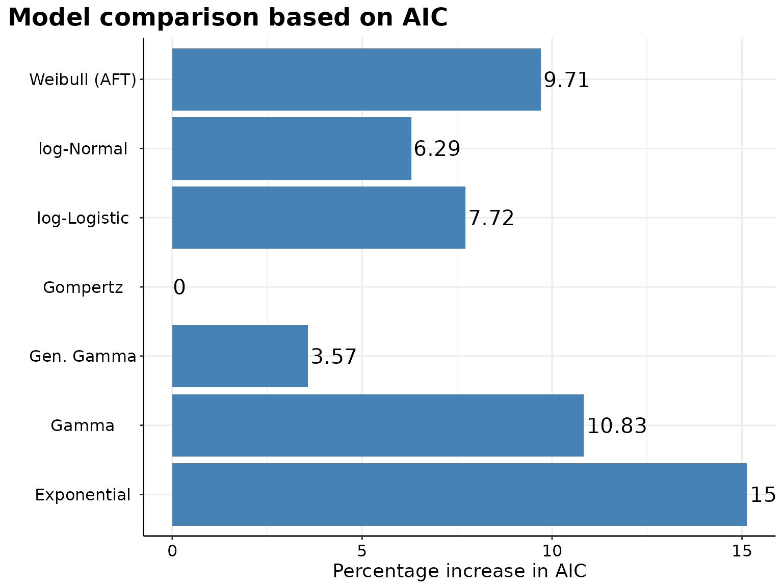
#>
#> Model fit for the Exponential model, obtained using Flexsurvreg
#> (Maximum Likelihood Estimate). Running time: 0.005 seconds
#>
#>           mean         se      L95%      U95%
#> rate 0.0529694 0.00727591 0.0404673 0.0693341
#>
#> Model fitting summaries
#> Akaike Information Criterion (AIC)....: 419.432
#> Bayesian Information Criterion (BIC)..: 422.151
#>
#>
#> Model fit for the Gamma model, obtained using Flexsurvreg
#> (Maximum Likelihood Estimate). Running time: 0.015 seconds
#>
#>            mean         se       L95%      U95%
#> shape 0.5484131 0.08420805 0.40588874 0.7409836
#> rate  0.0179479 0.00679396 0.00854672 0.0376899
#>
#> Model fitting summaries
#> Akaike Information Criterion (AIC)....: 403.768
#> Bayesian Information Criterion (BIC)..: 409.205
#>
#>
#> Model fit for the Generalised Gamma model, obtained using Flexsurvreg
#> (Maximum Likelihood Estimate). Running time: 0.025 seconds
#>
#>           mean       se      L95%      U95%
#> mu     1.01720 0.430972  0.172514  1.861894
#> sigma  2.17596 0.239791  1.753272  2.700562
#> Q     -1.90444 0.483808 -2.852686 -0.956192
#>
#> Model fitting summaries
#> Akaike Information Criterion (AIC)....: 377.339
#> Bayesian Information Criterion (BIC)..: 385.495
#>
#>
#> Model fit for the Gompertz model, obtained using Flexsurvreg
#> (Maximum Likelihood Estimate). Running time: 0.009 seconds
#>
#>            mean        se      L95%      U95%
#> shape -0.316976 0.0538467 -0.422513 -0.211438
#> rate   0.199665 0.0382986  0.137098  0.290787
#>
#> Model fitting summaries
#> Akaike Information Criterion (AIC)....: 364.319
#> Bayesian Information Criterion (BIC)..: 369.756
#>
#>
#> Model fit for the Weibull AF model, obtained using Flexsurvreg
#> (Maximum Likelihood Estimate). Running time: 0.005 seconds
#>
#>           mean        se     L95%      U95%
#> shape  0.59362 0.0737995  0.46525  0.757409
#> scale 27.22828 7.1596769 16.26285 45.587279
#>
#> Model fitting summaries
#> Akaike Information Criterion (AIC)....: 399.691
#> Bayesian Information Criterion (BIC)..: 405.128
#>
#>
#> Model fit for the log-Logistic model, obtained using Flexsurvreg
#> (Maximum Likelihood Estimate). Running time: 0.012 seconds
#>
#>            mean        se     L95%      U95%
#> shape  0.738167 0.0875116 0.585117  0.931251
#> scale 13.026802 3.3994377 7.811072 21.725260
#>
#> Model fitting summaries
#> Akaike Information Criterion (AIC)....: 392.443
#> Bayesian Information Criterion (BIC)..: 397.880
#>
#>
#> Model fit for the log-Normal model, obtained using Flexsurvreg
#> (Maximum Likelihood Estimate). Running time: 0.006 seconds
#>
#>            mean       se    L95%    U95%
#> meanlog 2.63022 0.265965 2.10894 3.15150
#> sdlog   2.22122 0.247771 1.78502 2.76402
#>
#> Model fitting summaries
#> Akaike Information Criterion (AIC)....: 387.246
#> Bayesian Information Criterion (BIC)..: 392.683
Fitting survival curves by treatment:
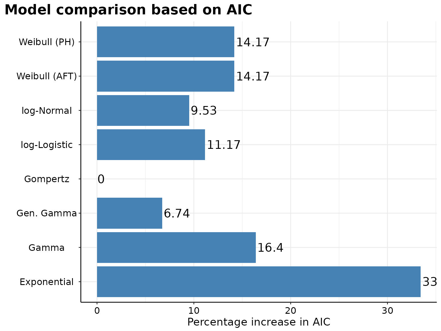
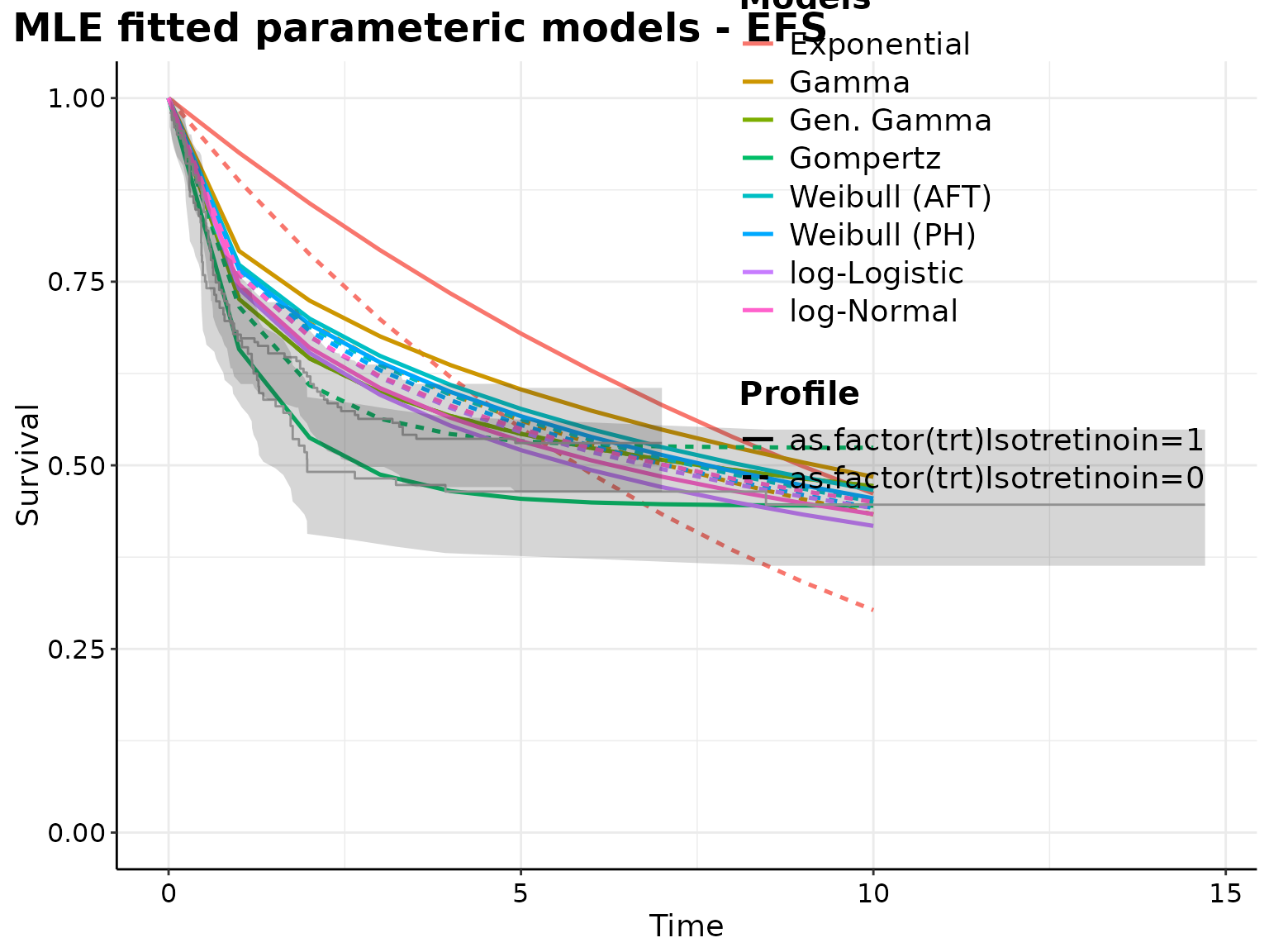
set.seed(1)
# Define models to be used
models <- c("exponential", "gamma", "gengamma", "gompertz", "weibull", "weibullPH", "loglogistic", "lognormal")

# Write formula specifying the predictor
formula <- survival::Surv(time = eventtime, event = event) ~ as.factor(trt)

# Fit parametric models:
parametric_models_trt <- lapply(
  X = names(IPD_curves) |>
    `names<-`(names(IPD_curves)),
  FUN = function(curves_nm) {
    surv_data <- IPD_curves[[curves_nm]]
    surv_parametric_models <- survHE::fit.models(
      formula = formula,
      data = surv_data,
      distr = models,
      method = "mle"
    )

    p <- survHE::model.fit.plot(
      surv_parametric_models,
      scale = "relative"
    )
    print(
      p +
        ggplot2::theme(
          plot.title.position = "plot",
          text = ggplot2::element_text(size = 10),
        )
    )

    p <- plot(surv_parametric_models, add.km = TRUE, t = seq(0, 10))
    print(
      p +
        ggplot2::labs(
          title = paste0(
            "MLE fitted parameteric models - ",
            gsub(
              pattern = "\\.",
              replacement = " ",
              curves_nm)
          )
        ) +
        ggplot2::theme(
          plot.title.position = "plot",
          # legend.text = ggplot2::element_text(size = 8),
          # legend.title = ggplot2::element_text(size = 8)
        )
    )

    lapply(
      X = seq_along(models),
      FUN = function(param_model) {
        print(surv_parametric_models, mod = param_model)
      }
    )

    surv_parametric_models
  }
)
#>
#> Model fit for the Exponential model, obtained using Flexsurvreg
#> (Maximum Likelihood Estimate). Running time: 0.008 seconds
#>
#>                                 mean        se       L95%      U95%
#> rate                        0.118862 0.0123922  0.0968946  0.145810
#> as.factor(trt)Isotretinoin -0.438358 0.1643125 -0.7604044 -0.116311
#>
#> Model fitting summaries
#> Akaike Information Criterion (AIC)....: 1022.332
#> Bayesian Information Criterion (BIC)..: 1029.818
#>
#>
#> Model fit for the Gamma model, obtained using Flexsurvreg
#> (Maximum Likelihood Estimate). Running time: 0.034 seconds
#>
#>                                  mean         se       L95%      U95%
#> shape                       0.4112712 0.03572089  0.3468944 0.4875950
#> rate                        0.0210414 0.00614059  0.0118759 0.0372807
#> as.factor(trt)Isotretinoin -0.2660013 0.31656550 -0.8864583 0.3544557
#>
#> Model fitting summaries
#> Akaike Information Criterion (AIC)....: 891.870
#> Bayesian Information Criterion (BIC)..: 903.099
#>
#>
#> Model fit for the Generalised Gamma model, obtained using Flexsurvreg
#> (Maximum Likelihood Estimate). Running time: 0.060 seconds
#>
#>                                   mean       se      L95%      U95%
#> mu                          0.28951910 0.398744 -0.492005  1.071043
#> sigma                       2.87338994 0.178113  2.544667  3.244577
#> Q                          -1.50188010 0.285066 -2.060599 -0.943161
#> as.factor(trt)Isotretinoin -0.00122724 0.349128 -0.685505  0.683051
#>
#> Model fitting summaries
#> Akaike Information Criterion (AIC)....: 817.839
#> Bayesian Information Criterion (BIC)..: 832.811
#>
#>
#> Model fit for the Gompertz model, obtained using Flexsurvreg
#> (Maximum Likelihood Estimate). Running time: 0.024 seconds
#>
#>                                 mean        se       L95%      U95%
#> shape                      -0.726308 0.0689758 -0.8614983 -0.591118
#> rate                        0.465813 0.0598415  0.3621262  0.599187
#> as.factor(trt)Isotretinoin  0.222220 0.1643144 -0.0998302  0.544271
#>
#> Model fitting summaries
#> Akaike Information Criterion (AIC)....: 766.230
#> Bayesian Information Criterion (BIC)..: 777.459
#>
#>
#> Model fit for the Weibull AF model, obtained using Flexsurvreg
#> (Maximum Likelihood Estimate). Running time: 0.008 seconds
#>
#>                                  mean        se      L95%      U95%
#> shape                       0.4708127 0.0338952  0.408853  0.542162
#> scale                      15.6867205 3.7969324  9.761148 25.209452
#> as.factor(trt)Isotretinoin  0.0847999 0.3514551 -0.604040  0.773639
#>
#> Model fitting summaries
#> Akaike Information Criterion (AIC)....: 874.771
#> Bayesian Information Criterion (BIC)..: 886.000
#>
#>
#> Model fit for the Weibull PH model, obtained using Flexsurvreg
#> (Maximum Likelihood Estimate). Running time: 0.008 seconds
#>
#>                                  mean        se      L95%     U95%
#> shape                       0.4708127 0.0338952  0.408853 0.542162
#> scale                       0.2736077 0.0313235  0.218615 0.342434
#> as.factor(trt)Isotretinoin -0.0399249 0.1658334 -0.364952 0.285103
#>
#> Model fitting summaries
#> Akaike Information Criterion (AIC)....: 874.771
#> Bayesian Information Criterion (BIC)..: 886.000
#>
#>
#> Model fit for the log-Logistic model, obtained using Flexsurvreg
#> (Maximum Likelihood Estimate). Running time: 0.008 seconds
#>
#>                                 mean        se      L95%      U95%
#> shape                       0.598128 0.0413215  0.522383  0.684855
#> scale                       6.577741 1.5502123  4.144474 10.439606
#> as.factor(trt)Isotretinoin -0.180774 0.3688524 -0.903711  0.542164
#>
#> Model fitting summaries
#> Akaike Information Criterion (AIC)....: 851.780
#> Bayesian Information Criterion (BIC)..: 863.009
#>
#>
#> Model fit for the log-Normal model, obtained using Flexsurvreg
#> (Maximum Likelihood Estimate). Running time: 0.011 seconds
#>
#>                                 mean       se      L95%     U95%
#> meanlog                     1.955391 0.239781  1.485429 2.425353
#> sdlog                       2.767214 0.178823  2.438015 3.140863
#> as.factor(trt)Isotretinoin -0.117646 0.357465 -0.818265 0.582973
#>
#> Model fitting summaries
#> Akaike Information Criterion (AIC)....: 839.272
#> Bayesian Information Criterion (BIC)..: 850.501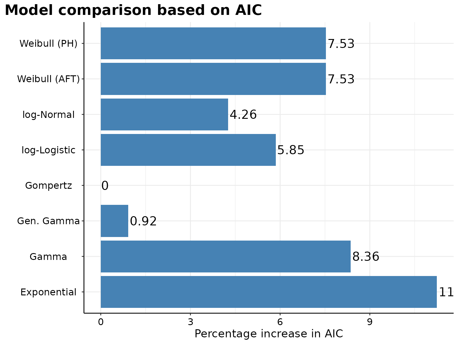
#>
#> Model fit for the Exponential model, obtained using Flexsurvreg
#> (Maximum Likelihood Estimate). Running time: 0.007 seconds
#>
#>                                  mean         se       L95%       U95%
#> rate                        0.0767895 0.00911324  0.0608531  0.0968994
#> as.factor(trt)Isotretinoin -0.3713533 0.18152805 -0.7271417 -0.0155649
#>
#> Model fitting summaries
#> Akaike Information Criterion (AIC)....: 927.902
#> Bayesian Information Criterion (BIC)..: 935.388
#>
#>
#> Model fit for the Gamma model, obtained using Flexsurvreg
#> (Maximum Likelihood Estimate). Running time: 0.034 seconds
#>
#>                                  mean         se      L95%      U95%
#> shape                       0.6181381 0.06159460  0.508472 0.7514565
#> rate                        0.0291709 0.00825689  0.016750 0.0508024
#> as.factor(trt)Isotretinoin -0.2484417 0.26148253 -0.760938 0.2640546
#>
#> Model fitting summaries
#> Akaike Information Criterion (AIC)....: 903.851
#> Bayesian Information Criterion (BIC)..: 915.080
#>
#>
#> Model fit for the Generalised Gamma model, obtained using Flexsurvreg
#> (Maximum Likelihood Estimate). Running time: 0.070 seconds
#>
#>                                  mean       se      L95%      U95%
#> mu                          0.7626838 0.294464  0.185546  1.339822
#> sigma                       2.1024632 0.163794  1.804741  2.449299
#> Q                          -2.2764560 0.384736 -3.030525 -1.522387
#> as.factor(trt)Isotretinoin -0.0180095 0.250363 -0.508711  0.472692
#>
#> Model fitting summaries
#> Akaike Information Criterion (AIC)....: 841.795
#> Bayesian Information Criterion (BIC)..: 856.767
#>
#>
#> Model fit for the Gompertz model, obtained using Flexsurvreg
#> (Maximum Likelihood Estimate). Running time: 0.017 seconds
#>
#>                                 mean        se      L95%      U95%
#> shape                      -0.359927 0.0460278 -0.450140 -0.269715
#> rate                        0.182694 0.0265867  0.137358  0.242994
#> as.factor(trt)Isotretinoin  0.189991 0.1824706 -0.167644  0.547627
#>
#> Model fitting summaries
#> Akaike Information Criterion (AIC)....: 834.131
#> Bayesian Information Criterion (BIC)..: 845.360
#>
#>
#> Model fit for the Weibull AF model, obtained using Flexsurvreg
#> (Maximum Likelihood Estimate). Running time: 0.007 seconds
#>
#>                                 mean        se      L95%      U95%
#> shape                       0.649354 0.0532257  0.552982  0.762521
#> scale                      20.941809 4.5328734 13.701586 32.007926
#> as.factor(trt)Isotretinoin  0.177736 0.2828866 -0.376711  0.732184
#>
#> Model fitting summaries
#> Akaike Information Criterion (AIC)....: 896.963
#> Bayesian Information Criterion (BIC)..: 908.192
#>
#>
#> Model fit for the Weibull PH model, obtained using Flexsurvreg
#> (Maximum Likelihood Estimate). Running time: 0.007 seconds
#>
#>                                 mean        se      L95%     U95%
#> shape                       0.649354 0.0532257  0.552982 0.762521
#> scale                       0.138738 0.0203823  0.104026 0.185032
#> as.factor(trt)Isotretinoin -0.115414 0.1853777 -0.478747 0.247920
#>
#> Model fitting summaries
#> Akaike Information Criterion (AIC)....: 896.963
#> Bayesian Information Criterion (BIC)..: 908.192
#>
#>
#> Model fit for the log-Logistic model, obtained using Flexsurvreg
#> (Maximum Likelihood Estimate). Running time: 0.008 seconds
#>
#>                                  mean        se      L95%      U95%
#> shape                       0.7782543 0.0609471  0.667516  0.907363
#> scale                      11.8431864 2.4415556  7.906557 17.739841
#> as.factor(trt)Isotretinoin  0.0529205 0.2974335 -0.530038  0.635879
#>
#> Model fitting summaries
#> Akaike Information Criterion (AIC)....: 882.954
#> Bayesian Information Criterion (BIC)..: 894.183
#>
#>
#> Model fit for the log-Normal model, obtained using Flexsurvreg
#> (Maximum Likelihood Estimate). Running time: 0.011 seconds
#>
#>                                 mean       se      L95%     U95%
#> meanlog                    2.5213424 0.210812  2.108158 2.934527
#> sdlog                      2.1388640 0.157040  1.852192 2.469906
#> as.factor(trt)Isotretinoin 0.0662944 0.288606 -0.499363 0.631952
#>
#> Model fitting summaries
#> Akaike Information Criterion (AIC)....: 869.654
#> Bayesian Information Criterion (BIC)..: 880.883
Best parametric model:
The Gompertz model seems to best fits the data and offers the best predictive performance for the survival curves of both interventions.
set.seed(1)
# Define models to be used
models <- "gompertz"

# Write formula specifying the predictor
formula <- survival::Surv(time = eventtime, event = event) ~ 1

# Fit parametric models:
parametric_models <- lapply(
  X = names(IPD_curves_trts) |>
    `names<-`(names(IPD_curves_trts)),
  FUN = function(curves_trts_nm) {
    surv_data <- IPD_curves_trts[[curves_trts_nm]]
    surv_parametric_models <- survHE::fit.models(
      formula = formula,
      data = surv_data,
      distr = models,
      method = "mle"
    )

    p <- plot(
      surv_parametric_models,
      add.km = TRUE,
      t = seq(0, 10),
      legend.position = "none"
    )
    print(
      p +
        ggplot2::coord_cartesian(xlim = c(0, 10)) +
        ggplot2::labs(
          title = paste0(
            "Gompertz fitted models - ",
            gsub(
              pattern = "\\.",
              replacement = " ",
              curves_trts_nm)
          )
        ) +
        ggplot2::theme(plot.title.position = "plot")
    )

    lapply(
      X = seq_along(models),
      FUN = function(param_model) {
        print(surv_parametric_models, mod = param_model)
      }
    )

    surv_parametric_models$models$Gompertz
  }
)
#>
#> Model fit for the Gompertz model, obtained using Flexsurvreg
#> (Maximum Likelihood Estimate). Running time: 0.011 seconds
#>
#>            mean        se      L95%      U95%
#> shape -0.771794 0.0969359 -0.961785 -0.581803
#> rate   0.488828 0.0706664  0.368217  0.648946
#>
#> Model fitting summaries
#> Akaike Information Criterion (AIC)....: 466.408
#> Bayesian Information Criterion (BIC)..: 473.004
#>
#> Model fit for the Gompertz model, obtained using Flexsurvreg
#> (Maximum Likelihood Estimate). Running time: 0.010 seconds
#>
#>            mean        se      L95%      U95%
#> shape -0.676088 0.0959712 -0.864188 -0.487988
#> rate   0.549287 0.0935185  0.393440  0.766867
#>
#> Model fitting summaries
#> Akaike Information Criterion (AIC)....: 301.333
#> Bayesian Information Criterion (BIC)..: 306.770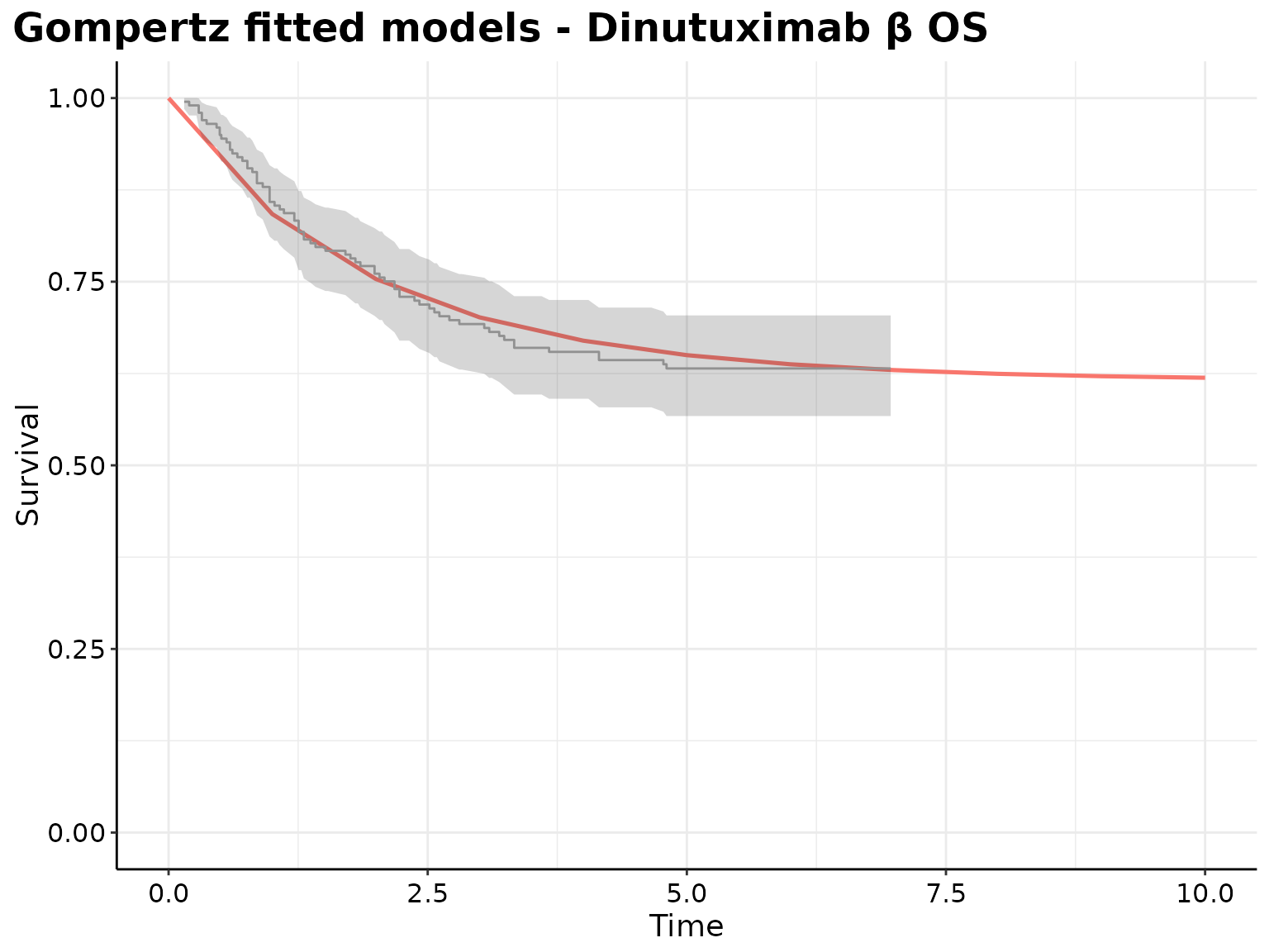
#>
#> Model fit for the Gompertz model, obtained using Flexsurvreg
#> (Maximum Likelihood Estimate). Running time: 0.011 seconds
#>
#>            mean        se      L95%      U95%
#> shape -0.437065 0.0785317 -0.590984 -0.283146
#> rate   0.208811 0.0365708  0.148141  0.294328
#>
#> Model fitting summaries
#> Akaike Information Criterion (AIC)....: 470.201
#> Bayesian Information Criterion (BIC)..: 476.797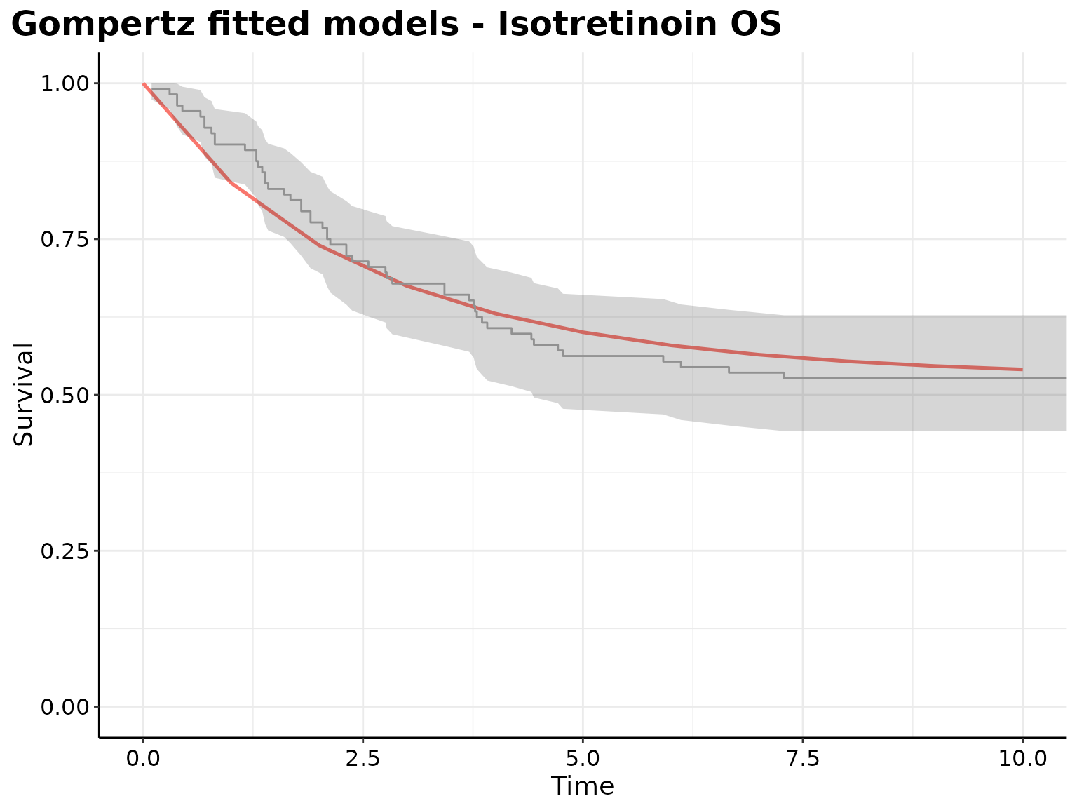
#>
#> Model fit for the Gompertz model, obtained using Flexsurvreg
#> (Maximum Likelihood Estimate). Running time: 0.010 seconds
#>
#>            mean        se      L95%      U95%
#> shape -0.316976 0.0538467 -0.422513 -0.211438
#> rate   0.199665 0.0382986  0.137098  0.290787
#>
#> Model fitting summaries
#> Akaike Information Criterion (AIC)....: 364.319
#> Bayesian Information Criterion (BIC)..: 369.756