Introduction:
A partitioned survival model (PSM) with N distinct states quantifies the likelihood of a patient occupying each of these states at any specific time, given a certain treatment. This model relies on overlapping survival curves to estimate state membership, requiring a total of N-1 such curves for an N-state configuration.
The model uses the cumulative survival function, , to define the chance of a patient either reaching or surpassing a certain health state after time . For the initial state, the probability is directly indicated by . The determination of membership for intermediate states, from the second to the , is achieved through the difference . The likelihood that a patient advances to the terminal state , often signifying death, is given by , essentially the complement of the cumulative survival up to the next-to-last state.
For each treatment strategy , the model predicts separate survival curves over time for each treatment approach and individual patient , based on parameters , which may be modified by covariates ,
Quality-adjusted life years (QALYs) and total costs for each health state, under a specific treatment and patient scenario, are derived by integrating the survival probability over time, adjusted by quality of life weights and costs. For any health state , the calculations for QALYs and costs in the costs category are represented as:
$$ \begin{aligned} \rm{QALYs}_{hik} &= \int_{0}^{T} q_{hik}(t) e^{-rt} p_{hik}(t)dt \\ \rm{Costs}_{m,hik} &= \int_{0}^{T} c_{m,hik}(t) e^{-rt} p_{hik}(t)dt \end{aligned} $$
Here, denotes the quality-of-life weight, represents annualized costs, stands for the discount rate, and signifies the probability of being in a specific health state at time . These calculations span over time periods to account for QALYs and associated costs.
The model:
Model parameters:
The model parameters include the time horizon of decision problem and states payoffs or rewards.
# Model parameters
params <- list()
params$time_horizon <- 10
params$cycles_per_year <- 12
params$c_TT  <- 2000 # place holder
params$c_GD2 <- 3000 # place holder
params$c_PPS <- 3200 # place holder
params$u_EFS <- 0.23 # place holder
params$u_PPS <- 0.23 # place holder
params$disc_rate <- 0.035
Survival curves:
The analysis documented by the Survival functions vignette suggests that Gompertz model fits the data best. The parameters of the fitted Gompertz distribution are employed in the section below to predict the cumulative survival curves over the model time horizon.
# Load the fitted `Gompertz` model parameters
models_fit <- NeuroblastomaPSM::parametric_models

# Get the months from 0 to time horizon
time_points <- seq(
  from = 0,
  to = params$time_horizon,
  by = 1 / params$cycles_per_year
)

# Predict cumulative survival
set.seed(1)
df_survival_curves_long <- lapply(
  X = names(models_fit) |>
    `names<-`(names(models_fit)),
  FUN = function(curve_nm) {
    model_fit <- models_fit[[curve_nm]]

    end_point <- ifelse(
      test = grepl(pattern = "OS", x = curve_nm),
      yes = "OS",
      no = "EFS"
    )

    treatment_nm <- gsub(
      pattern = paste0(".", end_point),
      replacement = "",
      x = curve_nm
    )

    NeuroblastomaPSM::predict_survival_curve(
      surv_mod = model_fit,
      treatment_name = treatment_nm,
      end_point = end_point,
      time_points = time_points
    )
  }
) |>
  do.call(
    what = rbind,
    args = _
  ) |>
  `rownames<-`(NULL)

# View predicted cumulative survival dataframe
rbind(
  head(df_survival_curves_long, n = 5),
  tail(df_survival_curves_long, n = 5)
)
#>     treatment end_point        time  survival
#> 1         GD2       EFS  0.00000000 1.0000000
#> 2         GD2       EFS  0.08333333 0.9613148
#> 3         GD2       EFS  0.16666667 0.9264001
#> 4         GD2       EFS  0.25000000 0.8948133
#> 5         GD2       EFS  0.33333333 0.8661732
#> 480        TT        OS  9.66666667 0.5485409
#> 481        TT        OS  9.75000000 0.5481205
#> 482        TT        OS  9.83333333 0.5477113
#> 483        TT        OS  9.91666667 0.5473131
#> 484        TT        OS 10.00000000 0.5469255
State membership (Markov trace):
This model is represented by three health states, event free survival (EFS), post progression survival (PPS) and death. Using the predicted EFS and OS, state membership is estimated below.
# Pivoting wider using reshape() - long-formatted to wide-formatted
df_survival_curves <- reshape(
  data = df_survival_curves_long,
  timevar = "end_point",
  idvar = c("time", "treatment"),
  direction = "wide"
)

# Renaming the columns since reshape() adds a prefix to the column names
names(df_survival_curves) <- gsub("survival\\.", "", names(df_survival_curves))

# Creating new columns
df_markov_trace <- df_survival_curves
df_markov_trace$PPS <- df_markov_trace$OS - df_markov_trace$EFS
df_markov_trace$D <- 1 - df_markov_trace$OS

# Selecting and ordering the desired columns (select in tidyverse)
df_markov_trace <- df_markov_trace[, c("time", "treatment", "EFS", "PPS", "D")]

# View wide formatted predicted cumulative survival dataframe
rbind(
  head(df_markov_trace, n = 5),
  tail(df_markov_trace, n = 5)
)
#>            time treatment       EFS        PPS          D
#> 1    0.00000000       GD2 1.0000000 0.00000000 0.00000000
#> 2    0.08333333       GD2 0.9613148 0.02174250 0.01694267
#> 3    0.16666667       GD2 0.9264001 0.04059241 0.03300746
#> 4    0.25000000       GD2 0.8948133 0.05693773 0.04824901
#> 5    0.33333333       GD2 0.8661732 0.07110898 0.06271787
#> 238  9.66666667        TT 0.4442937 0.10424725 0.45145908
#> 239  9.75000000        TT 0.4442650 0.10385549 0.45187954
#> 240  9.83333333        TT 0.4442379 0.10347342 0.45228872
#> 241  9.91666667        TT 0.4442122 0.10310083 0.45268695
#> 242 10.00000000        TT 0.4441880 0.10273749 0.45307451

# Confirm markov trace is valid
stopifnot(
  "Markov trace does not sum up to 1." =
    all(rowSums(df_markov_trace[, c("EFS", "PPS", "D")]) == 1)
)

# Visualize the markov trace
df_markov_trace |>
  reshape(
    data = _,
    varying = list(c("EFS", "PPS", "D")),
    v.names = "prop",
    timevar = "State",
    times = c("EFS", "PPS", "D"),
    direction = "long"
  ) |>
  ggplot2::ggplot(
    mapping = ggplot2::aes(
      x = time,
      y = prop,
      col = State
    )
  )+
  ggplot2::geom_step() +
  ggplot2::theme_classic() +
  ggplot2::scale_y_continuous(name = "Proportion") +
  ggplot2::scale_x_continuous(name = "Time (years)") +
  ggplot2::scale_color_manual(
    name = "State",
    values = c("D"= 1,
               "EFS" = 2,
               "PPS" = 3),
    labels = c("D"="Dead",
               "EFS" = "EFS",
               "PPS" = "PPS")
  ) +
  ggplot2::facet_wrap(~treatment)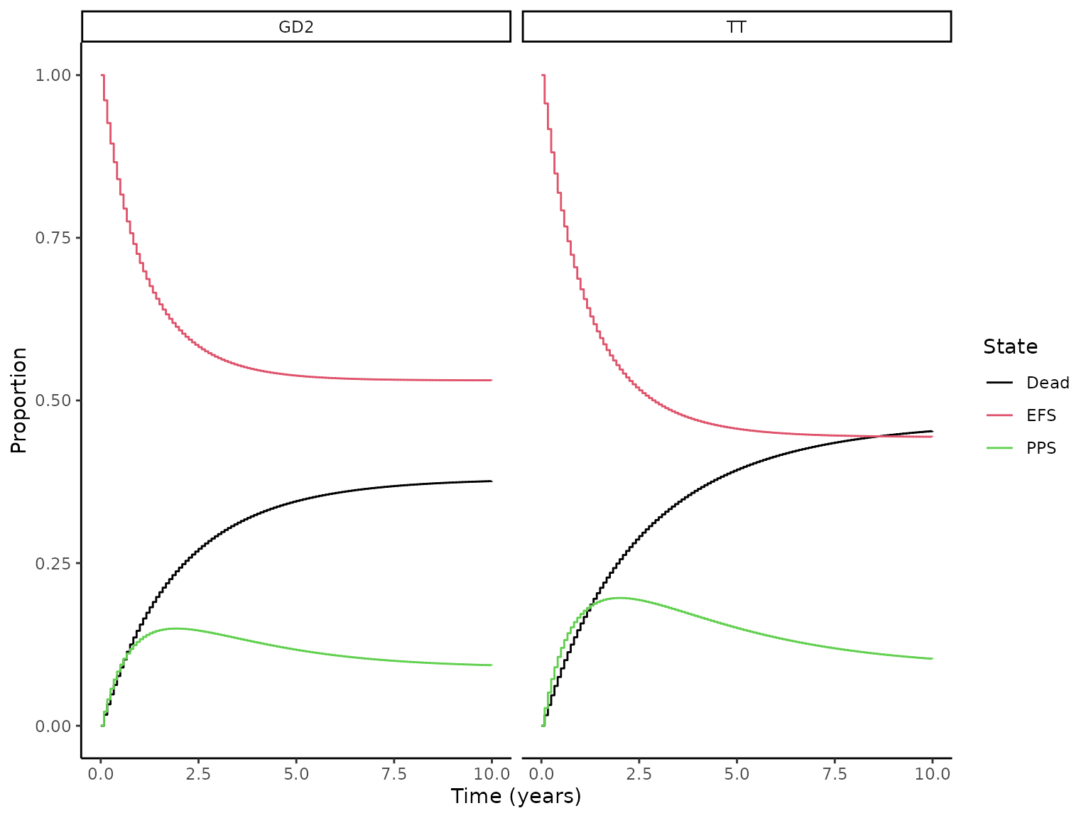
Economic Analysis:
# create matrices for matrix multiplication
m_TR_Isotretinoin <- as.matrix(
  df_markov_trace[
    df_markov_trace$treatment == "Isotretinoin", c("EFS", "PPS", "D")
  ]
)
m_TR_Dinutuximab_β <- as.matrix(
  df_markov_trace[
    df_markov_trace$treatment == "Dinutuximab β", c("EFS", "PPS", "D")
  ]
)

# create vectors of health states payoffs
v_C_Isotretinoin <- c("EFS" = params$c_TT,
                      "PPS" = params$c_PPS,
                      "D" = 0)

v_C_Dinutuximab_β <- c("EFS" = params$c_GD2,
                       "PPS" = params$c_PPS,
                       "D" = 0)
v_Util <- c("EFS" = params$u_EFS,
         "PPS" = params$u_PPS,
         "D" = 0)

# Matrix multiplication of trace by:
## cost per cycle - gives total cost by cycle
v_costs_Isotretinoin  <- m_TR_Isotretinoin %*%
  (v_C_Isotretinoin / params$cycles_per_year)
v_costs_Dinutuximab_β <- m_TR_Dinutuximab_β %*%
  (v_C_Dinutuximab_β / params$cycles_per_year)

## utility by cycle - gives total utility by cycle
v_qalys_Isotretinoin  <- m_TR_Isotretinoin %*%
  (v_Util / params$cycles_per_year)
v_qalys_Dinutuximab_β <- m_TR_Dinutuximab_β %*%
  (v_Util / params$cycles_per_year)

# Combine payoffs' calculations
m_results <- cbind(
  "c_Isotretinoin" = v_costs_Isotretinoin,
  "c_Dinutuximab_β" = v_costs_Dinutuximab_β,
  "q_Isotretinoin" = v_qalys_Isotretinoin,
  "q_Dinutuximab_β" = v_qalys_Dinutuximab_β
) |>
  `colnames<-`(c("c_Isotretinoin", "c_Dinutuximab_β", "q_Isotretinoin", "q_Dinutuximab_β"))

# Calculate discount weights
v_dw <- 1 /(1 + params$disc_rate) ^ time_points

# Apply discount weights to all columns of results matrix simultaneously
## this gives total discounted costs and qalys over the whole period.
m_disc_res <- v_dw %*% m_results |>
  `colnames<-`(c("c_Isotretinoin", "c_Dinutuximab_β", "q_Isotretinoin", "q_Dinutuximab_β"))

# Calculate incremental costs and utilities
inc_cost  <- m_disc_res[, "c_Dinutuximab_β"] - m_disc_res[, "c_Isotretinoin"]
inc_qaly  <- m_disc_res[, "q_Dinutuximab_β"] - m_disc_res[, "q_Isotretinoin"]

# calculate the ICER
as.numeric(inc_cost / inc_qaly)
#> numeric(0)