
Introduction:
As we discussed in a previous post, one of the main advantages of Application Programming Interfaces (API)s over web-based applications (such as the shiny-powered ones) is programmatic access. As the term suggests, programmatic access is or takes part in an automated process.
It might be challenging to picture this if we are new to programming. Therefore, this tutorial aims to demonstrate programmatic access to APIs.
So, in this post, we will:
- discuss the relevance to HTA,
- describe the API we will use,
- containerise the API using docker, and
- interact with the API programmatically.
Relevance, prerequisites and difficulty:
Relevance:
We have started discussing APIs and their relevance in a previous post. Nonetheless, one advantage of programmatic access is that it enables the integration of different tools or programming languages into the analysis process.
Difficulty:
We rank this tutorial as intermediate owing to the background knowledge and skills it builds upon and the technical bits it covers.
Prerequisites:
We expect those who intend to follow along to understand the basics of plumber-powered APIs (please see here for a quick recap).
Moreover, we need the software:
- R,
- RStudio, and
- Docker.
We will jump between R and Visual Studio Code (VS code) Integrated Development Environments (IDE)s. Having VS code in our systems would ease the process, but it is unnecessary for this tutorial.
The files containing the code we demonstrate below are hosted here. Once we have cloned this repository, using the git clone command, we need to open PowerShell from within the “posts” folder to ensure that the commands demonstrated below work on our systems.
The API:
Smith et al. (2022)1 covered the usefulness of APIs in general and their applications in the Health Technology Appraisal (HTA) domain. Also, the authors provide an example API that:
- controls access to some fictitious data, allowing cleared users to pass their decision-analytic model code to the API hosting infrastructure,
- processes the code, and
- responds with the outputs of the analysis.
We use the code provided by Smith et al. (2022) in the following parts of this post. We advise those interested in learning more about the API to consult the paper.
Containerising the API:
As we have discussed in a previous post, containerising APIs helps ease the deployment process. Below we demonstrate building a plumber-equipped docker image and copying the API files into it. We start by displaying the dockerfile that will generate the API image.
1
2
3
4
5
6
7
8
9
10
11
12
13
14
# Dockerfile

# Get the docker image provided by plumber developers:
FROM rstudio/plumber
# Install the R package `pacman`:
RUN R -e "install.packages('pacman')"
# Use pacman to install other required packages:
RUN R -e "pacman::p_load('assertthat', 'dampack', 'ggplot2', 'jsonlite', 'readr')"
# Create a working directory in the container:
WORKDIR /api
# Copy API files to the created working directory in the container:
COPY ./RobertASmithBresMed-plumberHE-809f204/darthAPI /api
# Specify the commands to run once the container runs:
CMD ["/api/plumber.R"]
In the third and fourth instructions in this dockerfile, we instruct docker to install essential R packages as part of the build process. Now, to build an image from the above dockerfile, we call:
1
docker build --tag living_hta:1.0 --file .\interacting-with-a-plumber-powered-API-programmatically\Dockerfile .\interacting-with-a-plumber-powered-API-programmatically
Note that we downloaded the API files from here and extracted them into the “deploying-plumber-powered-APIs-with-docker” folder. If it is unclear, the “.\interacting-with-a-plumber-powered-API-programmatically” part of the build child command is to let docker know that this is the context (scope) in which it should look to complete the COPY instruction.
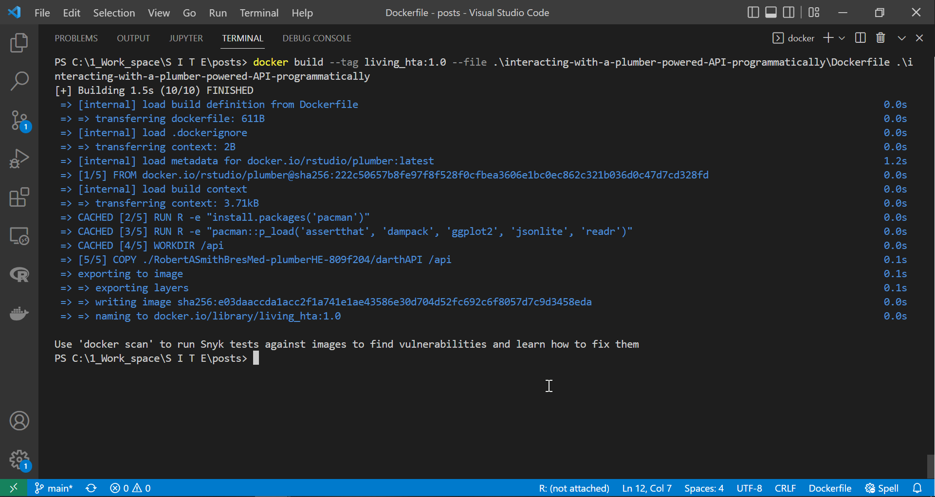 |
|---|
| Building the API image |
Once docker completes the build process, we can check if the container is running correctly by spinning it on attached mode. This way, we can observe the container outputs for any immediate errors or issues preventing the API from running.
1
2
# Run it in the foreground (keep access to the container's inputs and outputs):
docker run -p 8080:8000 -it --rm --name living_hta_api living_hta:1.0
 |
|---|
| Running the API container in attached mode |
As we can see in the screen recording above, we successfully deployed the plumber API in the container. However, unlike the suggestion made by the plumber at the end above gif, we would not get access to the API if we tried to access the documentation page at “http://127.0.0.1:8000/docs/”. This event is because containers are isolated from the host machine unless we specify otherwise. Therefore, since we exposed or linked port 8080 on our device to port 8000 on the container, this containerised API documentation is accessible here “http://127.0.0.1:8080/docs/”.
 |
|---|
| Accessing hosted API documentation |
Interacting with the API programmatically:
We have covered most of the previously discussed points in a previous tutorial; therefore, let us interact with the API programmatically. There are a few ways to perform this, but we will focus on the way that seems most natural in our HTA context. Below we utilise R, RStudio and the package httr. While httr plays a vital role in the following examples, we will only cover the functions relevant to the example(s) we present below.
httr is an R wrapper for curl and provides functions for the most commonly used HTTP verbs (read more about these methods in Smith et al. (2022)), namely: GET(), HEAD(), PATCH(), PUT(), DELETE() and POST(). That is enough introduction about httr, so let us see it in action.
Below we use httr’s POST function to send a request to the plumber-powered API, and we use httr’s content function to handle the returned response. But what arguments are we passing to the request (or request object) generator function POST()?
- url: this argument defines the domain or, in our example, the “local host address” of the API host
http://127.0.0.1and the port8080through which we can communicate with the API. - path: this argument names the endpoint to which we want the request to go.
- query and body: these arguments contain the data or information we want to pass along the request. Datasets, or data frames in this example, are usually passed through the body argument.
1
2
3
4
5
6
7
8
9
10
11
12
13
14
15
16
17
18
19
20
21
22
results <- httr::content(
  httr::POST(
    # the Server URL can also be kept confidential, but will leave here for now:
    url = "http://127.0.0.1:8080",
    # path for the API within the server URL:
    path = "/runDARTHmodel",
    # code is passed to the client API from GitHub:
    query = list(
        model_functions =
                   paste0("https://raw.githubusercontent.com/",
                          "BresMed/plumberHE/main/R/darth_funcs.R")),
    # set of parameters to be changed:
    body = list(
      param_updates = jsonlite::toJSON(
        data.frame(parameter = c("p_HS1","p_S1H"),
                   distribution = c("beta","beta"),
                   v1 = c(25, 50),
                   v2 = c(150, 100))
      )
    )
  )
)
As indicated earlier, the POST function creates the request object, whereas contents() processes the results object returned by the API. We will return to the request object and the information it contains in a future post, but we advise interested readers to check this page for further details.
We demonstrate running the above code from RStudio after spinning up the container. We can see the container (or R running inside the container) reacting to the request sent from the R session running on our local machine. The parameters’ dataframe we passed to the body argument of POST() triggers this reaction.
 |
|---|
Sending requests to API and handling response via httr |
It might not be so obvious, but we are calling POST() from within content() to pass the former’s results to the latter. This clarification should naturally lead to the conclusion that piping (or %>%) POST() to content() also works.
1
2
3
4
5
6
7
8
9
10
11
12
13
14
15
16
17
18
# remember to load a package that exports the pipe "%>%":
results <- httr::POST(
  # the Server URL can also be kept confidential, but will leave here for now:
  url = "http://127.0.0.1:8080",
  # path for the API within the server URL:
  path = "/runDARTHmodel",
  # code is passed to the client API from GitHub:
  query = list(model_functions =
                 paste0("https://raw.githubusercontent.com/",
                        "BresMed/plumberHE/main/R/darth_funcs.R")),
  # set of parameters to be changed:
  body = list(
    param_updates = jsonlite::toJSON(
      data.frame(parameter = c("p_HS1","p_S1H"),
                 distribution = c("beta","beta"),
                 v1 = c(25, 50),
                 v2 = c(150, 100))))) %>%
  httr::content()
Let us build on the API query above to demonstrate a higher level of programmatic access than just auto-sending code and data to the API and auto-processing the generated response. Below we pass the dataframe generated from processing the response object to colMeans() to get the average costs and consequences predicted by the simulation.
1
2
3
4
5
6
7
8
9
10
11
12
13
14
15
16
17
18
19
# remember to load a package that exports the pipe "%>%":
results <- httr::POST(
  # the Server URL can also be kept confidential, but will leave here for now:
  url = "http://127.0.0.1:8080",
  # path for the API within the server URL:
  path = "/runDARTHmodel",
  # code is passed to the client API from GitHub:
  query = list(model_functions =
                 paste0("https://raw.githubusercontent.com/",
                        "BresMed/plumberHE/main/R/darth_funcs.R")),
  # set of parameters to be changed:
  body = list(
    param_updates = jsonlite::toJSON(
      data.frame(parameter = c("p_HS1","p_S1H"),
                 distribution = c("beta","beta"),
                 v1 = c(25, 50),
                 v2 = c(150, 100))))) %>%
  httr::content() %>%
  colMeans()
We can see in the gif file below that the container is running successfully and reacting to the requests we are sending. Also, notice that the name of the terminal on the top right corner of the VS code window is docker, indicating that we are still connected to the container we span earlier.
 |
|---|
| API request and response blend seamlessly within the script |
Okay, but so far, we have not seen how the automation of this process is significantly valuable. To help us illustrate this point, we employ the contents of the “run_darthAPI.R” script (displayed below), which utilises the outputs of the above code to summarise the simulation results and compile an RMarkdown report automatically. First, however, we make two changes to the url and path arguments in the script to correctly direct its request to the locally hosted API; we comment out the existing url and post statements (using #) and add the ones we used in the above code chunk.
1
2
3
4
5
6
7
8
9
10
11
12
13
14
15
16
17
18
19
20
21
22
23
24
25
26
27
28
29
30
31
32
33
34
35
36
37
38
39
40
41
42
43
44
45
46
47
48
# remove all existing data from the environment.
rm(list = ls())

library(ggplot2)
library(jsonlite)
library(httr)

# run the model using the connect server API
results <- httr::content(
  httr::POST(
    # the Server URL can also be kept confidential, but will leave here for now
    #url = "https://connect.bresmed.com",
    url = "http://127.0.0.1:8080",
    # path for the API within the server URL
    #path = "rhta2022/runDARTHmodel",
    path = "/runDARTHmodel",
    # code is passed to the client API from GitHub.
    query = list(model_functions =
                   paste0("https://raw.githubusercontent.com/",
                          "BresMed/plumberHE/main/R/darth_funcs.R")),
    # set of parameters to be changed ...
    # we are allowed to change these but not some others
    body = list(
      param_updates = jsonlite::toJSON(
        data.frame(parameter = c("p_HS1","p_S1H"),
                   distribution = c("beta","beta"),
                   v1 = c(25, 50),
                   v2 = c(150, 100))
      )
    ),
    # we include a key here to access the API ... like a password protection
    config = httr::add_headers(Authorization = paste0("Key ",
                                                      Sys.getenv("CONNECT_KEY")))
  )
)

# write the results as a csv to the outputs folder...
write.csv(x = results,
          file = "outputs/darth_model_results.csv")

source("report/makeCEAC.R")
source("report/makeCEPlane.R")

# render the markdown document from the report folder,
# passing the results dataframe to the report.
rmarkdown::render(input = "report/darthreport.Rmd",
                  params = list("df_results" = results),
                  output_dir = "outputs")
We did not discuss the config argument of the httr::POST function, but we will cover it in our next plumber-related tutorial. However, we only highlight that this argument adds information to the request object, but we are not using it here.
Conclusion:
This short tutorial discussed a few examples of programmatic interaction with APIs. While the scenarios covered in this post concerned a plumber-powered API, we can extend programmatic access via R scripts to almost all APIs.
Sources:
Smith RA, Schneider PP and Mohammed W. Living HTA: Automating Health Economic Evaluation with R. Wellcome Open Res 2022, 7:194 (https://doi.org/10.12688/wellcomeopenres.17933.2). ↩